Experimenting to optimize SQL query by x360 and some tips to read query plans

Introducing the schema

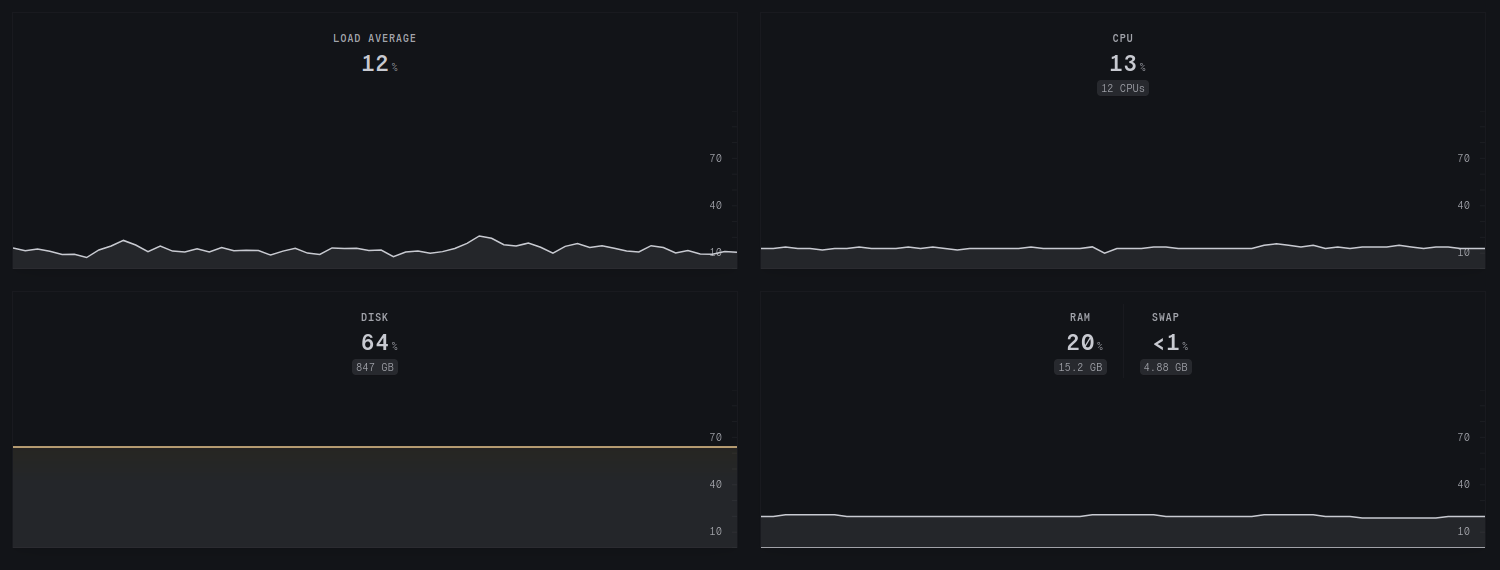
RorVsWild stores server metrics each minute (load average, CPU, memory and storage). The table has few millions of entries and weight a bit less than 2GB. That is neither huge nor small, but it is big enough to cause slow queries if something is wrong with indexes. And as we are monitoring RorVsWild with RorVsWild, we cannot ignore something wrong here.

The slow query returns data to display a chart of the load average from several servers. The chart displays 3 lines: the minimum, the maximum, and the average. That is useful for detecting if one server is out of breath or slacking.

This data comes from the table server_metrics_per_minutes with the following definition:

\d server_metrics_per_minutes
                                           Table "public.server_metrics_per_minutes"
    Column     |              Type              | Collation | Nullable |                        Default
---------------+--------------------------------+-----------+----------+--------------------------------------------------------
 id            | bigint                         |           | not null | nextval('server_metrics_per_minutes_id_seq'::regclass)
 server_id     | bigint                         |           | not null |
 -- Columns which are not relevant have been removed
 load_average  | double precision               |           | not null |
 cpu_count     | integer                        |           |          |
 created_at    | timestamp(6) without time zone |           | not null |
 updated_at    | timestamp(6) without time zone |           | not null |
Indexes:
    "server_metrics_per_minutes_pkey" PRIMARY KEY, btree (id)
    "index_server_metrics_per_minutes_on_created_at_and_server_id" btree (created_at, server_id)
    "index_server_metrics_per_minutes_on_server_id_and_created_at" UNIQUE, btree (server_id, date_trunc('minute'::text, created_at))
Foreign-key constraints:
    "fk_rails_c12a7f2f44" FOREIGN KEY (server_id) REFERENCES servers(id)

The table stores a row per server and per minute with the load average and the CPU count. Other columns have been redacted since we don’t need them for this article. The second index, a unique index, server_id, date_trunc('minute'::text, created_at), ensures only one metric per server is stored. It is not intended to optimize readings but only to guarantee uniqueness.

The next step is to explore the slow query.

The slow query

WITH intervals AS (
  SELECT date AS from_date, date + INTERVAL '1 minutes' AS to_date
  FROM GENERATE_SERIES('2025-02-16T14:00:00', '2025-02-16T15:00:00', INTERVAL '1 minutes') AS date
)
SELECT
  from_date,
  to_date,
  avg(load_average / cpu_count * 100) AS avg,
  min(load_average / cpu_count * 100) AS min,
  max(load_average / cpu_count * 100) AS max
FROM intervals
LEFT OUTER JOIN server_metrics_per_minutes
  ON server_id IN (229201, 22378, 22381, 229200)
  AND created_at BETWEEN from_date AND to_date
GROUP BY from_date, to_date
ORDER BY from_date;

The query returns a row for each minute between 2025-02-16T14:00:00 and 2025-02-16T15:00:00 across four servers. Each row has two timestamps and the three load average values for the selected servers.

It starts with a common table expression that is used to join on each minute. It contains 61 rows, one per minute, thanks to generate_series. Thus, the query returns a row even if there are no metrics. Without this trick, displaying the chart would have been awkward if some data had been missing.

The join condition uses indexed columns server_id IN (229201, 22378, 22381, 229200) AND created_at BETWEEN from_date AND to_date, so everything seems optimized.

Before making any changes, the first step is to inspect the query plan. It tells all the steps across tables and indexes used by the database. It’s best to enable the option ANALYZE to get actual timings instead of estimations. With ANALYZE, it becomes like a profiler. With Ruby on Rails, you can get quickly obtain the query plan for any combination of scopes by calling the ActiveRecord method explain: Model.scope1.scope2.explain(:analyze). Note that explain accepts options since version 7.1 only.

Let’s go back to the plan of the query explained above:

Understanding the query plan

                                                                                                 QUERY PLAN
------------------------------------------------------------------------------------------------------------------------------------------------------------------------------------------------------------
 Sort  (cost=9447449.21..9447449.71 rows=200 width=40) (actual time=4372.648..4372.653 rows=61 loops=1)
   Sort Key: date.date
   Sort Method: quicksort  Memory: 29kB
   ->  HashAggregate  (cost=9447438.57..9447441.57 rows=200 width=40) (actual time=4372.605..4372.625 rows=61 loops=1)
         Group Key: date.date, (date.date + '00:01:00'::interval)
         Batches: 1  Memory Usage: 48kB
         ->  Nested Loop Left Join  (cost=5499.93..7962688.03 rows=42421444 width=28) (actual time=851.288..4371.978 rows=244 loops=1)
               Join Filter: ((server_metrics_per_minutes.created_at >= date.date) AND (server_metrics_per_minutes.created_at <= (date.date + '00:01:00'::interval)))
               Rows Removed by Join Filter: 21222876
               ->  Function Scan on generate_series date  (cost=0.00..10.00 rows=1000 width=8) (actual time=248.014..248.071 rows=61 loops=1)
               ->  Materialize  (cost=5499.93..221718.90 rows=381793 width=20) (actual time=1.465..27.781 rows=347920 loops=61)
                     ->  Bitmap Heap Scan on server_metrics_per_minutes  (cost=5499.93..219809.93 rows=381793 width=20) (actual time=89.370..460.398 rows=347920 loops=1)
                           Recheck Cond: (server_id = ANY ('{229201,22378,22381,229200}'::bigint[]))
                           Heap Blocks: exact=171735
                           ->  Bitmap Index Scan on index_server_metrics_per_minutes_on_server_id_and_created_at  (cost=0.00..5404.48 rows=381793 width=0) (actual time=49.403..49.404 rows=347920 loops=1)
                                 Index Cond: (server_id = ANY ('{229201,22378,22381,229200}'::bigint[]))
 Planning Time: 0.465 ms
 JIT:
   Functions: 18
   Options: Inlining true, Optimization true, Expressions true, Deforming true
   Timing: Generation 2.936 ms, Inlining 32.362 ms, Optimization 138.900 ms, Emission 76.837 ms, Total 251.035 ms
 Execution Time: 4379.703 ms
(22 rows)

4379ms is really too slow. My goal is to have a server reponse time below 500ms. If you add netwrok latency, the page should be loaded in 1s or less. It’s not instantaneous, but at least the user doesn’t have the frustration of waiting. So the maximum time for that query should be 100ms to let some room for other queries and views.

Query plans are often rough to read, and this one is no exception. The trap is to read the query plan from the first to the last line. It’s draining. It’s like watching a movie from the end to the beginning. You understand nothing until the beginning, which is discouraging. By the way, Memento is a good movie.

Fortunately, I have a heuristic to find the bottleneck most of the time easily. I look for the slowest step and the last lines.

The slowest step can be spotted with the most extended timing time=851.288..4371.978:

Nested Loop Left Join  (cost=5499.93..7962688.03 rows=42421444 width=28) (actual time=851.288..4371.978 rows=244 loops=1)
   Join Filter: ((server_metrics_per_minutes.created_at >= date.date) AND (server_metrics_per_minutes.created_at <= (date.date + '00:01:00'::interval)))
   Rows Removed by Join Filter: 21222876

There are a few things that I don’t like to see in a query plan:

• Nested loop
• Join Filters
• 21222876 Rows Removed by Join Filter

21222876 rows have been removed with a filter! Either the index has not been used, or PostgreSQL scanned a large portion of the table. There is an index issue, that we will resolve later.

Let’s move directly to the last lines, which are, in fact, the first step.

->  Bitmap Index Scan on index_server_metrics_per_minutes_on_server_id_and_created_at  (cost=0.00..5404.48 rows=381793 width=0) (actual time=49.403..49.404 rows=347920 loops=1)
    Index Cond: (server_id = ANY ('{229201,22378,22381,229200}'::bigint[]))

The multicolumn index on server_id, date_trunc('minute'::text, created_at) is used when it’s supposed to read the other on (created_at, server_id). Moreover, it uses only the first column as the Index Cond shows. Filtering on date range is done by the slowest step, which removes too many rows, as seen earlier. But why is PostgreSQL using the wrong index?

When I ask myself this question, 99% of the time, it’s my fault, and the other 1% it’s because statistics have not been updated. Let’s try to understand what is wrong in the query.

Experimentation to overcome ignorance

If you are a database expert, you probably already know why, but I’m just a Ruby on Rails developer. When I’m clueless, I run experiments. Changing the input and observing different outputs helps to understand how a system works. That could be changing a parameter, or doing the same thing in a different way. I do that even if the change seems silly and even though I think I know the result. Sometimes we can really be surprised! Among all experiments, this one caught my eye:

EXPLAIN ANALYZE SELECT
  date_trunc('minute', created_at),
  avg(load_average / cpu_count * 100) AS avg,
  min(load_average / cpu_count * 100) AS min,
  max(load_average / cpu_count * 100) AS max
FROM server_metrics_per_minutes
WHERE server_id IN (229201, 22378, 22381, 229200) AND created_at BETWEEN '2025-02-16T14:00:00' AND '2025-02-16T15:00:00'
GROUP BY date_trunc('minute', created_at)
ORDER BY date_trunc('minute', created_at);
                                                                                                              QUERY PLAN
---------------------------------------------------------------------------------------------------------------------------------------------------------------------------------------------------------------------------------------
 GroupAggregate  (cost=289.69..294.24 rows=91 width=32) (actual time=2.876..2.963 rows=60 loops=1)
   Group Key: (date_trunc('minute'::text, created_at))
   ->  Sort  (cost=289.69..289.92 rows=91 width=20) (actual time=2.863..2.878 rows=240 loops=1)
         Sort Key: (date_trunc('minute'::text, created_at))
         Sort Method: quicksort  Memory: 43kB
         ->  Index Scan using index_server_metrics_per_minutes_on_created_at_and_server_id on server_metrics_per_minutes  (cost=0.43..286.73 rows=91 width=20) (actual time=0.034..2.763 rows=240 loops=1)
               Index Cond: ((created_at >= '2025-02-16 14:00:00'::timestamp without time zone) AND (created_at <= '2025-02-16 15:00:00'::timestamp without time zone) AND (server_id = ANY ('{229201,22378,22381,229200}'::bigint[])))
 Planning Time: 0.266 ms
 Execution Time: 3.014 ms
(9 rows)

It’s the same query without the common table expression and the generate_series, but it ran in 3ms instead of 4379ms. The last step shows that the query planner is using the most relevant index on (server_id, created_at). That is why it’s a lot faster.

It’s great because I’m close to the solution. After some thinking, I finally came to the conclusion that PostgreSQL could not use the index on (created_at, server_id) because the GENERATE_SERIES('2025-02-16T14:00:00', '2025-02-16T15:00:00', INTERVAL '1 minutes') returns 61 timestamps. Indeed, that would require going through the index 61 times, and merging those 61 results. So, the query planner estimated that this a slower path.

Pre-filtering with the index

From here, we have all the knowledge to optimize the query. Rows must be pre-filtered by date range to allow the query planner to utilize the multicolumn index. Thus, the slowest step of the query has fewer lines to work on. Here is the one condition added to the original query:

 WITH intervals AS (
   SELECT date AS from_date, date + INTERVAL '1 minutes' AS to_date
   FROM GENERATE_SERIES('2025-02-16T14:00:00', '2025-02-16T15:00:00', INTERVAL '1 minutes') AS date
 )
 SELECT
   from_date,
   to_date,
   avg(load_average / cpu_count * 100) AS avg,
   min(load_average / cpu_count * 100) AS min,
   max(load_average / cpu_count * 100) AS max
 FROM intervals
 LEFT OUTER JOIN server_metrics_per_minutes
   ON server_id IN (229201, 22378, 22381, 229200)
   AND created_at BETWEEN from_date AND to_date
+  AND created_at BETWEEN '2025-02-16T14:00:00' AND '2025-02-16T15:00:00'
 GROUP BY from_date, to_date
 ORDER BY from_date;

Without knowing the whole story, it must look awkward to have two conditions created_at BETWEEN X AND Y. But as the query plan shows, it allows PostgreSQL to use the multicolumn index:

 Sort  (cost=2506.34..2506.84 rows=200 width=40) (actual time=11.748..11.756 rows=61 loops=1)
   Sort Key: date.date
   Sort Method: quicksort  Memory: 29kB
   ->  HashAggregate  (cost=2495.70..2498.70 rows=200 width=40) (actual time=11.682..11.711 rows=61 loops=1)
         Group Key: date.date, (date.date + '00:01:00'::interval)
         Batches: 1  Memory Usage: 48kB
         ->  Nested Loop Left Join  (cost=0.44..2141.81 rows=10111 width=28) (actual time=0.073..11.465 rows=241 loops=1)
               Join Filter: ((server_metrics_per_minutes.created_at >= date.date) AND (server_metrics_per_minutes.created_at <= (date.date + '00:01:00'::interval)))
               Rows Removed by Join Filter: 14400
               ->  Function Scan on generate_series date  (cost=0.00..10.00 rows=1000 width=8) (actual time=0.020..0.031 rows=61 loops=1)
               ->  Materialize  (cost=0.43..286.76 rows=91 width=20) (actual time=0.001..0.104 rows=240 loops=61)
                     ->  Index Scan using index_server_metrics_per_minutes_on_created_at_and_server_id on server_metrics_per_minutes  (cost=0.43..286.30 rows=91 width=20) (actual time=0.043..4.660 rows=240 loops=1)
                           Index Cond: ((created_at >= '2025-02-16 14:00:00'::timestamp without time zone) AND (created_at <= '2025-02-16 15:00:00'::timestamp without time zone) AND (server_id = ANY ('{229201,22378,22381,229200}'::bigint[])))
 Planning Time: 0.574 ms
 Execution Time: 11.877 ms
(15 rows)

The query is down from 4379ms to 11.87ms, which is 368 times faster! That is not bad for a single line added.

The first step (last lines) confirms that the multicolumn index on (created_at, server_id) is used on both columns. The query plan still shows Nested loop and Join filter but at least the removed rows decreased from 21222876 to 14400. So, the pre-filtering works great.

Conclusion

Query plans are rough to read, but their help is invaluable for optimizing queries. It becomes much easier with some tricks, such as looking for the slowest step or directly the last lines. When you’re clueless, experimentation is a good way to help you understand. Finally, pre-filtering has been the solution to decrease a lot the number of rows read by PostgreSQL.